MATLAB Six Bar Kinematic System
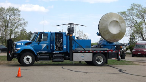
Parametric MATLAB model that computes and animates a six bar mechanism; demo shows a rotating Doppler-radar truck transitioning from driving to scanning orientation.

Overview & Simulation Context
This project involved developing a parametric MATLAB model to analyze and simulate the kinematics of a planar six-bar linkage. The mechanism was modeled in the context of a mobile Doppler radar truck, where a rotating mechanical linkage transitions the radar assembly between a driving configuration and an elevated scanning position. The goal of the simulation was to translate theoretical kinematic principles into a functional computational tool capable of calculating motion and visualizing system behavior over time.

Using user-defined geometric parameters and an input rotation, the model computes angular position, angular velocity, and angular acceleration for each linkage, as well as the resulting linear position, velocity, and acceleration of key points on the system. The final output includes both quantitative data and an animated visualization of the mechanism’s motion.
System Setup & Kinematic Model
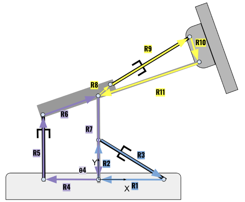
The system is modeled as a constrained planar six-bar linkage with fixed pivots, rotating links, and dependent joints. Each link length, joint location, and reference angle is explicitly defined, allowing the mechanism geometry to be adjusted parametrically. Loop-closure relationships are used to enforce kinematic constraints between connected links.
A labeled schematic of the linkage identifies each link, joint, and reference angle used in the analysis and serves as the foundation for the position, velocity, and acceleration calculations performed in MATLAB.
Computational Approach (MATLAB Implementation)
The kinematic analysis is implemented entirely in MATLAB without reliance on pre-built mechanism toolboxes. Position analysis is performed using trigonometric relationships derived from loop-closure equations. Angular velocity and angular acceleration are then calculated analytically by differentiating the position equations with respect to time.
The program is structured to progress logically from input definition to calculation to visualization. Arrays are used to store time-varying values for angular position, velocity, acceleration, and corresponding linear quantities. Modular code sections separate geometry setup, kinematic calculations, plotting routines, and animation logic, improving readability, debugging efficiency, and reusability.
Simulation & Animation Results
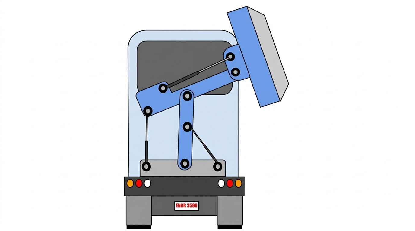
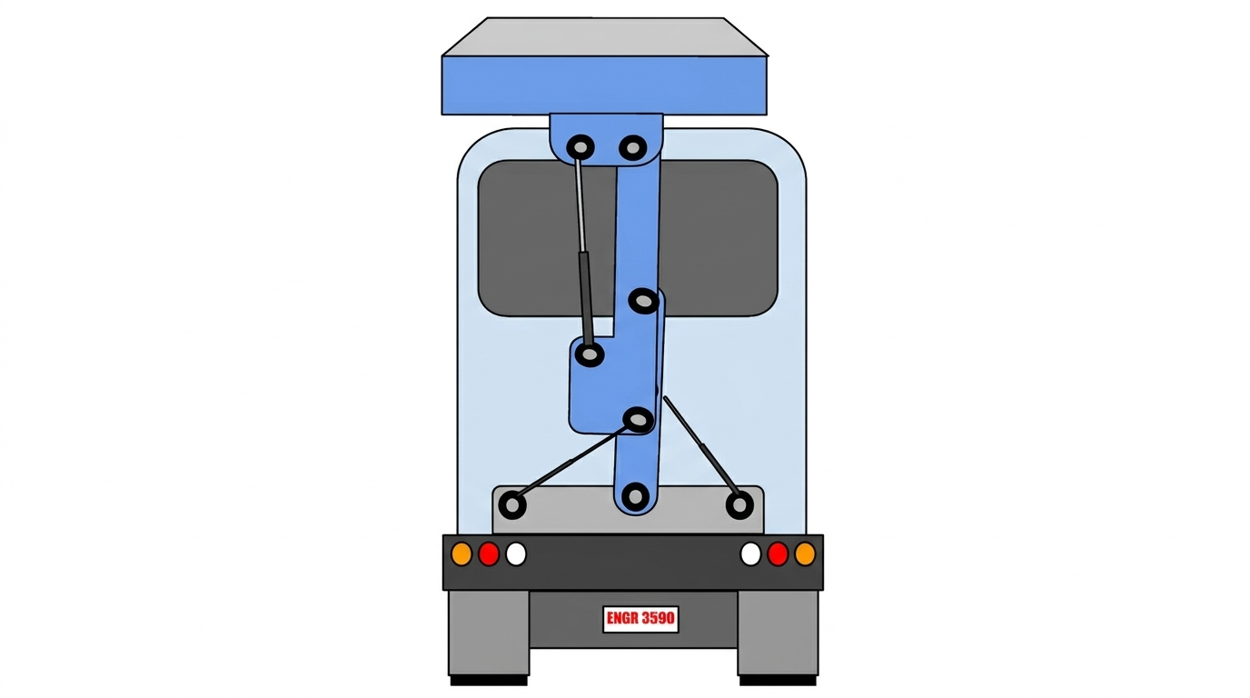
An animated visualization of the six-bar mechanism is generated to demonstrate the continuous motion of the system over a full input rotation cycle. The animation shows the radar structure smoothly transitioning between configurations, validating the correctness of the kinematic relationships and constraints.
Still frames from the animation highlight key positions throughout the motion cycle. A full video of the simulation is available through the linked demonstration.


Data Visualization & Output Graphs
In addition to animation, the model produces graphical outputs for angular and linear kinematic quantities. These include plots of angular position, angular velocity, and angular acceleration, as well as linear displacement, velocity, and acceleration of selected points on the mechanism.
Three-dimensional plots are used where appropriate to visualize how motion variables evolve simultaneously with respect to time and configuration. These visualizations provide insight into dynamic trends, peak accelerations, and regions of rapid motion that may influence mechanical design decisions.

This plot shows the time history of joint angles for the six-bar, three-loop mechanism as link length r₃ varies. It illustrates how changes in the input geometry propagate through the system and affect the relative angular positions of each joint.

This plot presents the angular velocities of each joint over time for the r₃ input case. The results highlight how motion introduced at the input link distributes dynamically across the coupled mechanism.

This plot shows the angular accelerations of the joints as a function of time for the r₃ configuration. These results provide insight into dynamic loading and regions of higher inertial demand within the multi-loop system.
Learning Outcomes & Engineering Takeaways
This project reinforced my understanding of planar kinematics and the relationship between theoretical equations and real mechanical motion. Beyond the mathematics, it strengthened my ability to structure computational code, debug geometric constraints, and present complex motion in a clear and visual format.
Most importantly, this experience demonstrated how an abstract mechanical concept can be transformed into a complete engineering deliverable — combining mathematical modeling, software implementation, and visual communication. The project deepened my confidence in using MATLAB as an engineering tool and highlighted the value of computational simulation in validating mechanical designs before physical prototyping.